Prior to identifying critical issues for the Southeast assessment focuses for the Fourth National Climate Assessment (NCA4), the Chapter Lead (CL) contacted numerous professional colleagues representing various geographic areas (e.g., Florida, Louisiana, and South Carolina) for expert opinions on critical climate change related issues impacting the region, with a particular emphasis on emerging issues since the Third National Climate Assessment (NCA3) effort.77 Following those interviews, the CL concluded that the most pressing climate change issues to focus on for the NCA4 effort were extreme events, flooding (both from rainfall and sea level rise), wildfire, health issues, ecosystems, and adaptation actions. Authors with specific expertise in each of these areas were sought, and a draft outline built around these issues was developed. Further refinement of these focal areas occurred in conjunction with the public Regional Engagement Workshop, held on the campus of North Carolina State University in March 2017 and in six satellite locations across the Southeast region. The participants agreed that the identified issues were important and suggested the inclusion of several other topics, including impacts on coastal and rural areas and people, forests, and agriculture. Based on the subsequent authors’ meeting and input from NCA staff, the chapter outline and Key Messages were updated to reflect a risk-based framing in the context of a new set of Key Messages. The depth of discussion for any particular topic and Key Message is dependent on the availability of supporting literature and chapter length limitations.
Key Message 1: Urban Infrastructure and Health Risks
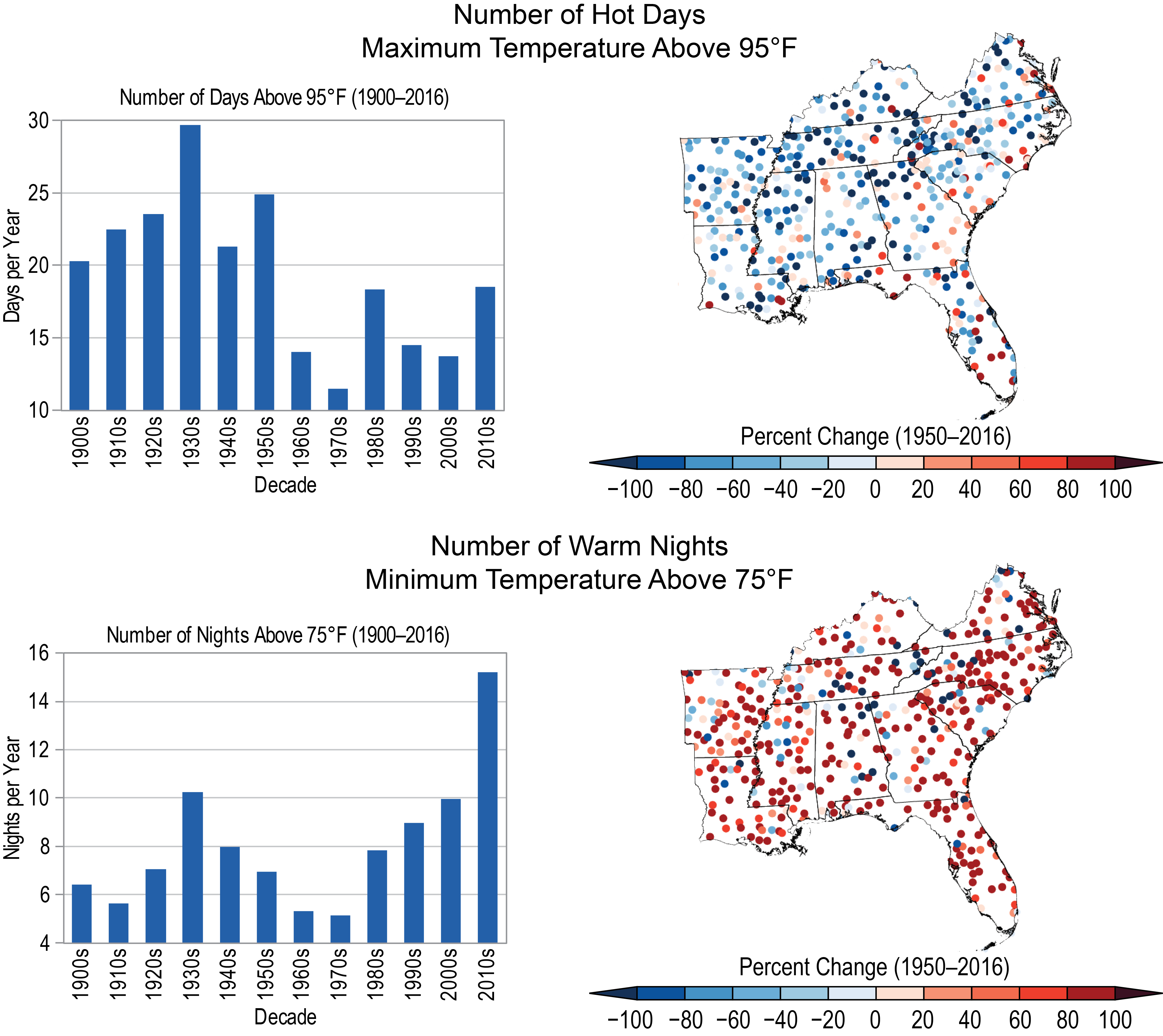
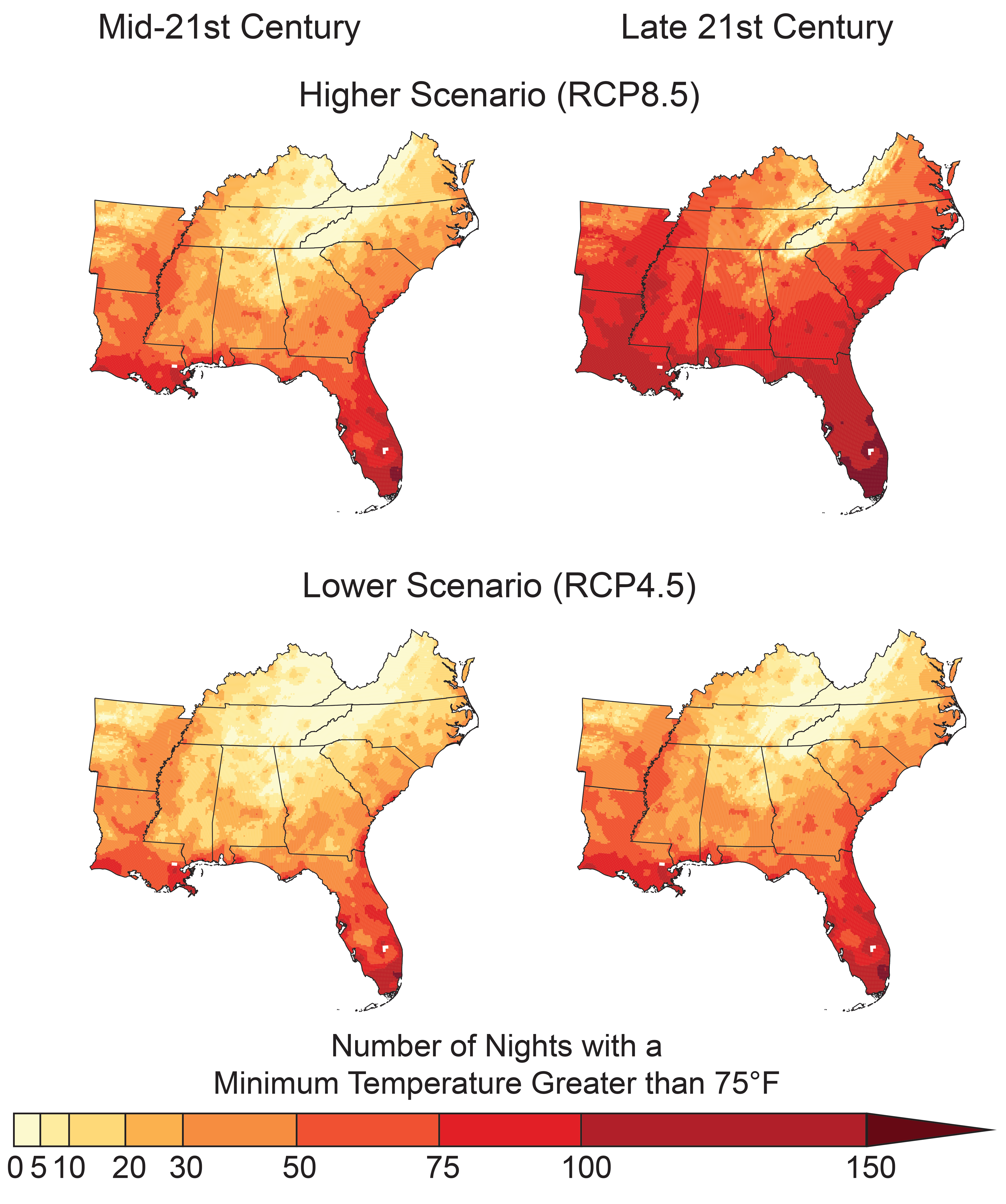
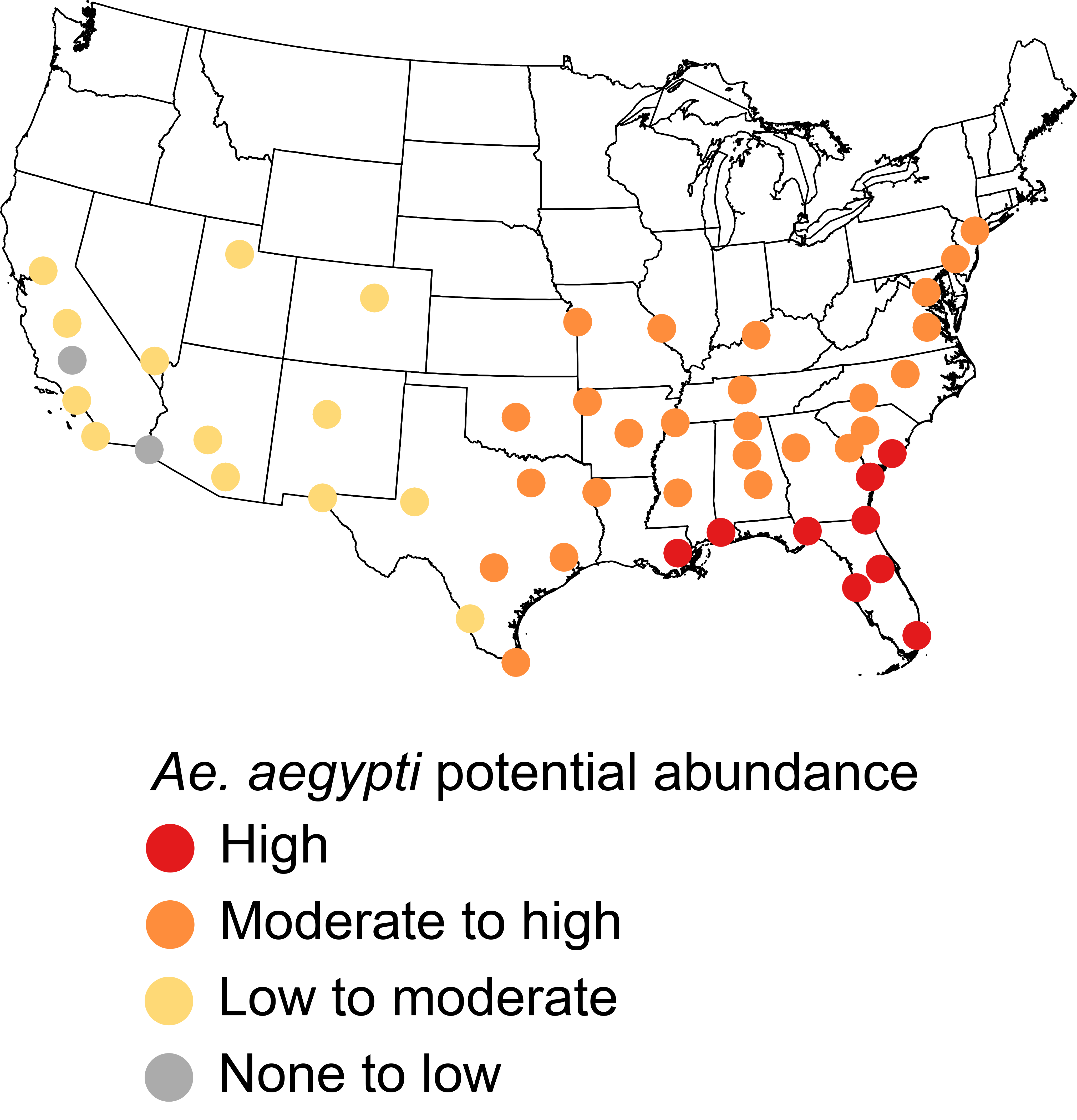
Many southeastern cities are particularly vulnerable to climate change compared to cities in other regions, with expected impacts to infrastructure and human health (very likely, very high confidence). The vibrancy and viability of these metropolitan areas, including the people and critical regional resources located in them, are increasingly at risk due to heat, flooding, and vector-borne disease brought about by a changing climate (likely, high confidence). Many of these urban areas are rapidly growing and offer opportunities to adopt effective adaptation efforts to prevent future negative impacts of climate change (very likely, high confidence).
Description of evidence base
Multiple studies have projected that urban areas, including those in the Southeast, will be adversely affected by climate change in a variety of ways. This includes impacts on infrastructure41,42,43,291,292,293 and human health.30,31,38,294 Increases in climate-related impacts have already been observed in some Southeast metropolitan areas (e.g., Habeeb et al. 2015, Tzung-May Fu et al. 201512,39).
Southeastern cities may be more vulnerable than cities in other regions of the United States due to the climate being more conducive to some vector-borne diseases, the presence of multiple large coastal cities at low elevation that are vulnerable to flooding and storms, and a rapidly growing urban and coastal population.22,295,296
Many city and county governments, utilities, and other government and service organizations have already begun to plan and prepare for the impacts of climate change (e.g., Gregg et al. 2017.; FTA 2013; City of Fayetteville 2017; City of Charleston 2015; City of New Orleans 2015; Tampa Bay Water 2014; EPA 2015; City of Atlanta 2015, 2017; Southeast Florida Regional Climate Change Compact 201744,45,46,50,91,246,297,298,299). A wide variety of adaptation options are available, offering opportunities to improve the climate resilience, quality of life, and economy of urban areas.77,300,301,302,303,304
Major uncertainties
Population projections are inherently uncertain over long time periods, and shifts in immigration or migration rates and shifting demographics will influence urban vulnerabilities to climate change. The precise impacts on cities are difficult to project. The scope and scale of adaptation efforts, which are already underway, will affect future vulnerability and risk. Technological developments (such as a potential shift in transportation modes) will also affect the scope and location of risk within cities. Newly emerging pathogens could increase risk of disease in the future, while successful adaptations could reduce public health risk.
Description of confidence and likelihood
There is very high confidence that southeastern cities will likely be impacted by climate change, especially in the areas of infrastructure and human health.
Key Message 2: Increasing Flood Risks in Coastal and Low-Lying Regions
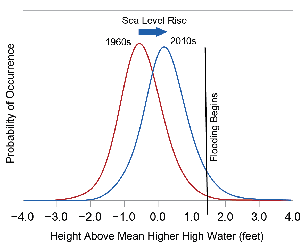
The Southeast’s coastal plain and inland low-lying regions support a rapidly growing population, a tourism economy, critical industries, and important cultural resources that are highly vulnerable to climate change impacts (very likely, very high confidence). The combined effects of changing extreme rainfall events and sea level rise are already increasing flood frequencies, which impacts property values and infrastructure viability, particularly in coastal cities. Without significant adaptation measures, these regions are projected to experience daily high tide flooding by the end of the century (likely, high confidence).
Description of evidence base
Multiple lines of research have shown that global sea levels have increased in the past and are projected to continue to accelerate in the future due to increased global temperature and that higher local sea level rise rates in the Mid-Atlantic and Gulf Coasts have occurred.51,52,53,54,55,56,57,59,61,62
Annual occurrences of high tide flooding have increased, causing several Southeast coastal cities to experience all-time records of occurrences that are posing daily risks.1,52,58,60,61,63,67,68
There is scientific consensus that sea level rise will continue to cause increases in high tide flooding in the Southeast as well as impact the frequency and duration of extreme water level events, causing an increase in the vulnerability of coastal populations and property.1,60,63,67,68
In the future, coastal flooding is projected to become more serious, disruptive, and costly as the frequency, depth, and inland extent grow with time.1,2,35,64,65,67,68
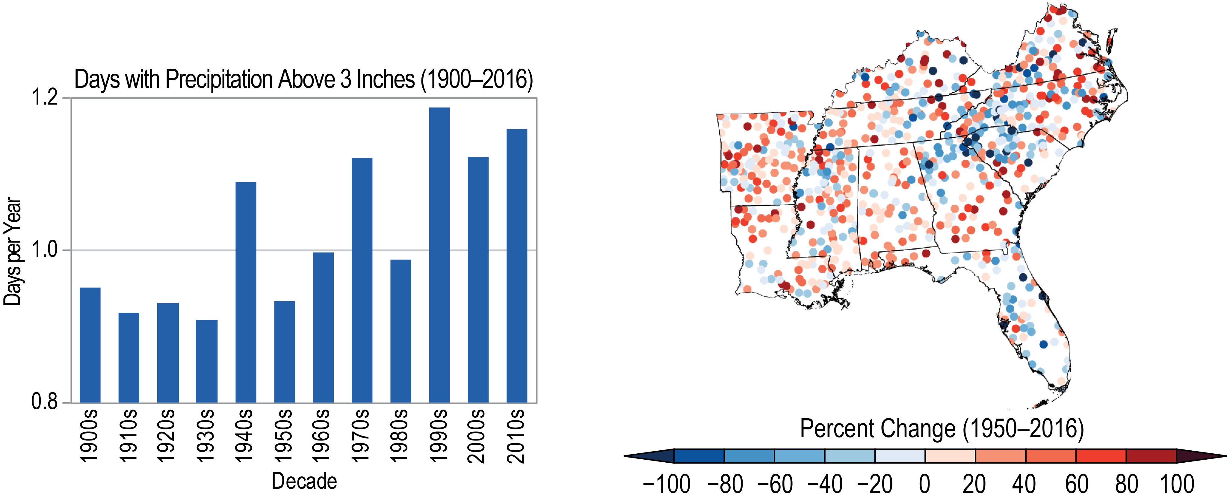
Many analyses have determined that extreme rainfall events have increased in the Southeast, and under higher scenarios, the frequency and intensity of these events are projected to increase.19,21,88
Rainfall records have shown that since NCA3, many intense rainfall events (approaching 500-year events) have occurred in the Southeast, with some causing billions of dollars in damage and many deaths.68,82,84
The flood events in Baton Rouge, Louisiana, in 2016 and in South Carolina in 2015 provide real examples of how vulnerable inland and coastal communities are to extreme rainfall events.81,85,86
The socioeconomic impacts of climate change on the Southeast is a developing research field.65,71
Major uncertainties
The amount of confidence associated with the historical rate of global sea level rise is impacted by the sparsity of tide gauge records and historical proxies as well as different statistical approaches for estimating sea level change. The amount of unpredictability in future projected rates of sea level rise is likely caused by a range of future climate scenarios projections and rate of ice sheet mass changes. Flooding events are highly variable in both space and time. Detection and attribution of flood events are difficult due to multiple variables that cause flooding.
Description of confidence and likelihood
There is high confidence that flood risks will very likely increase in coastal and low-lying regions of the Southeast due to rising sea level and an increase in extreme rainfall events. There is high confidence that Southeast coastal cities are already experiencing record numbers of high tide flooding events, and without significant adaptation measures, it is likely they will be impacted by daily high tide flooding.
Key Message 3: Natural Ecosystems Will Be Transformed
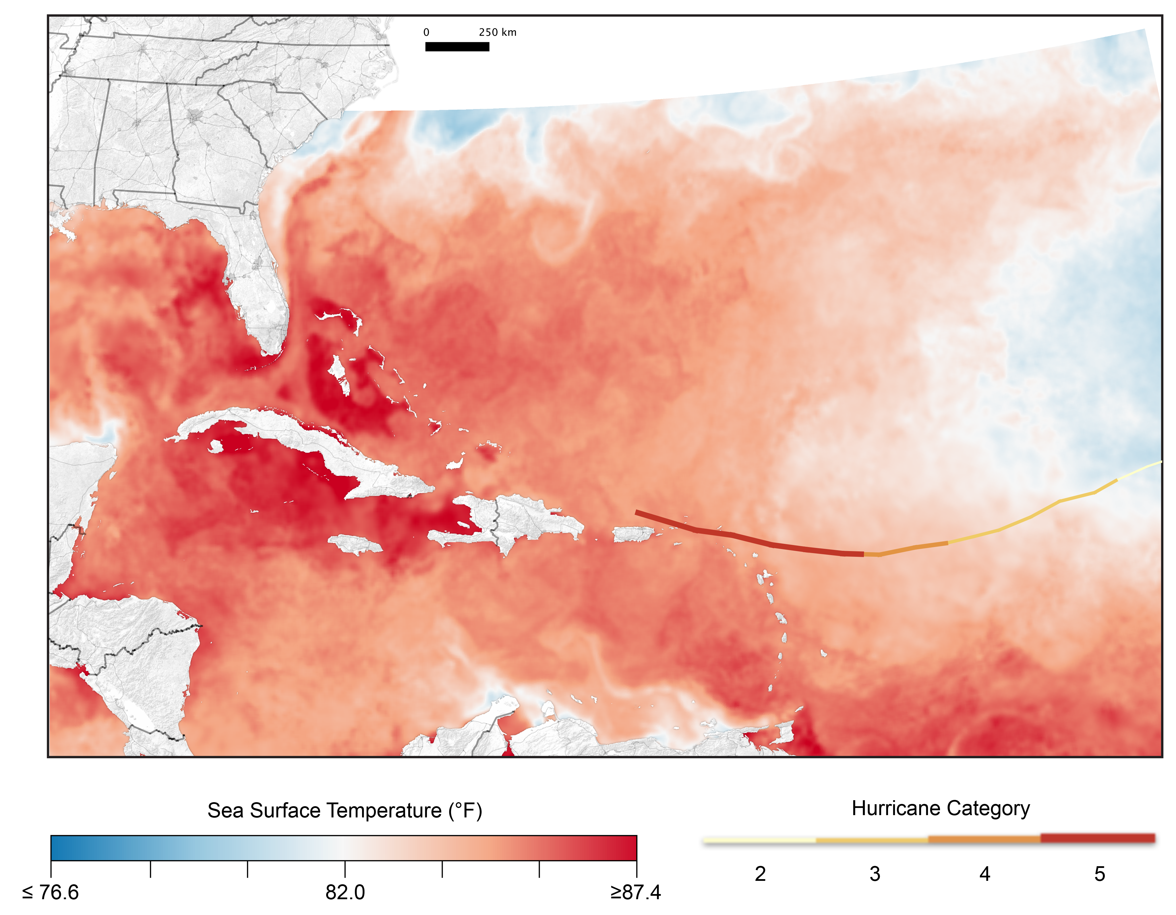
The Southeast’s diverse natural systems, which provide many benefits to society, will be transformed by climate change (very likely, high confidence). Changing winter temperature extremes, wildfire patterns, sea levels, hurricanes, floods, droughts, and warming ocean temperatures are expected to redistribute species and greatly modify ecosystems (very likely, high confidence). As a result, the ecological resources that people depend on for livelihood, protection, and well-being are increasingly at risk, and future generations can expect to experience and interact with natural systems that are much different than those that we see today (very likely, high confidence).
Description of evidence base
Winter temperature extremes, fire regimes, sea levels, hurricanes, rainfall extremes, drought extremes, and warming ocean temperatures greatly influence the distribution, abundance, and performance of species and ecosystems.
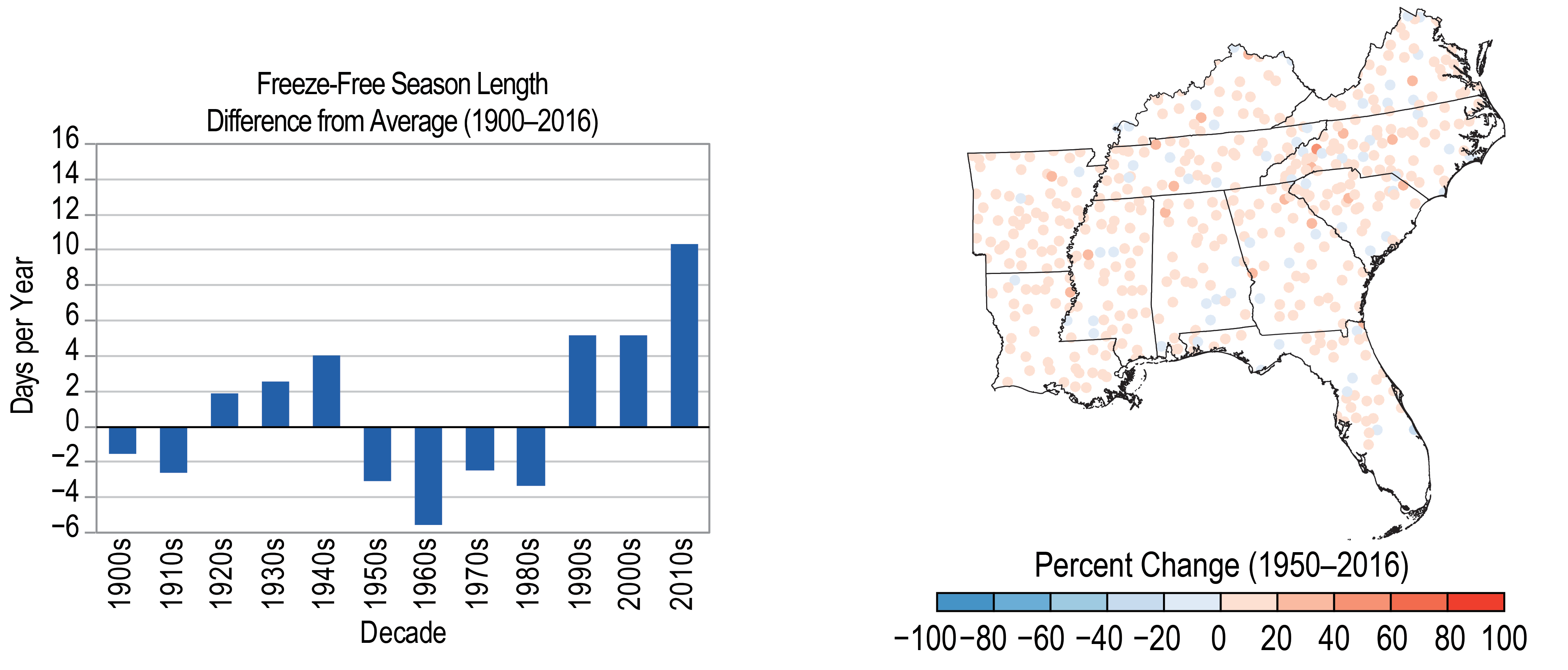
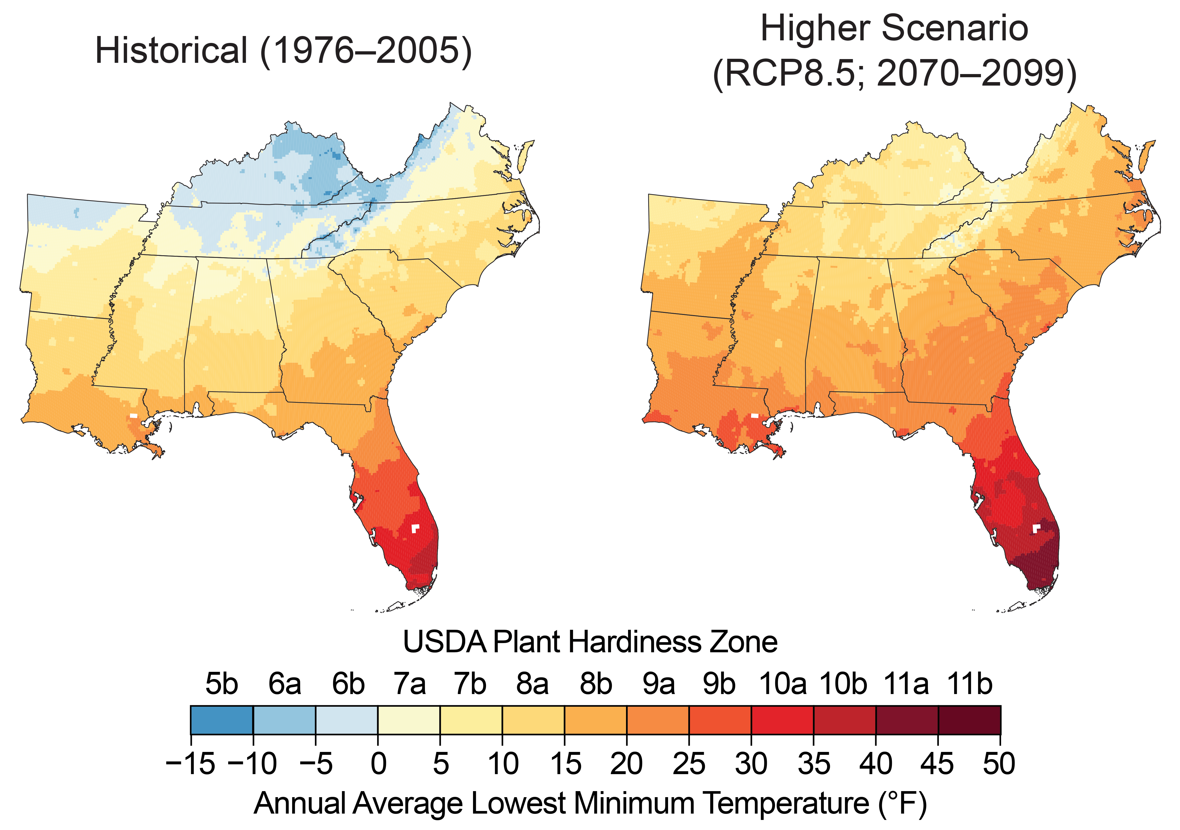
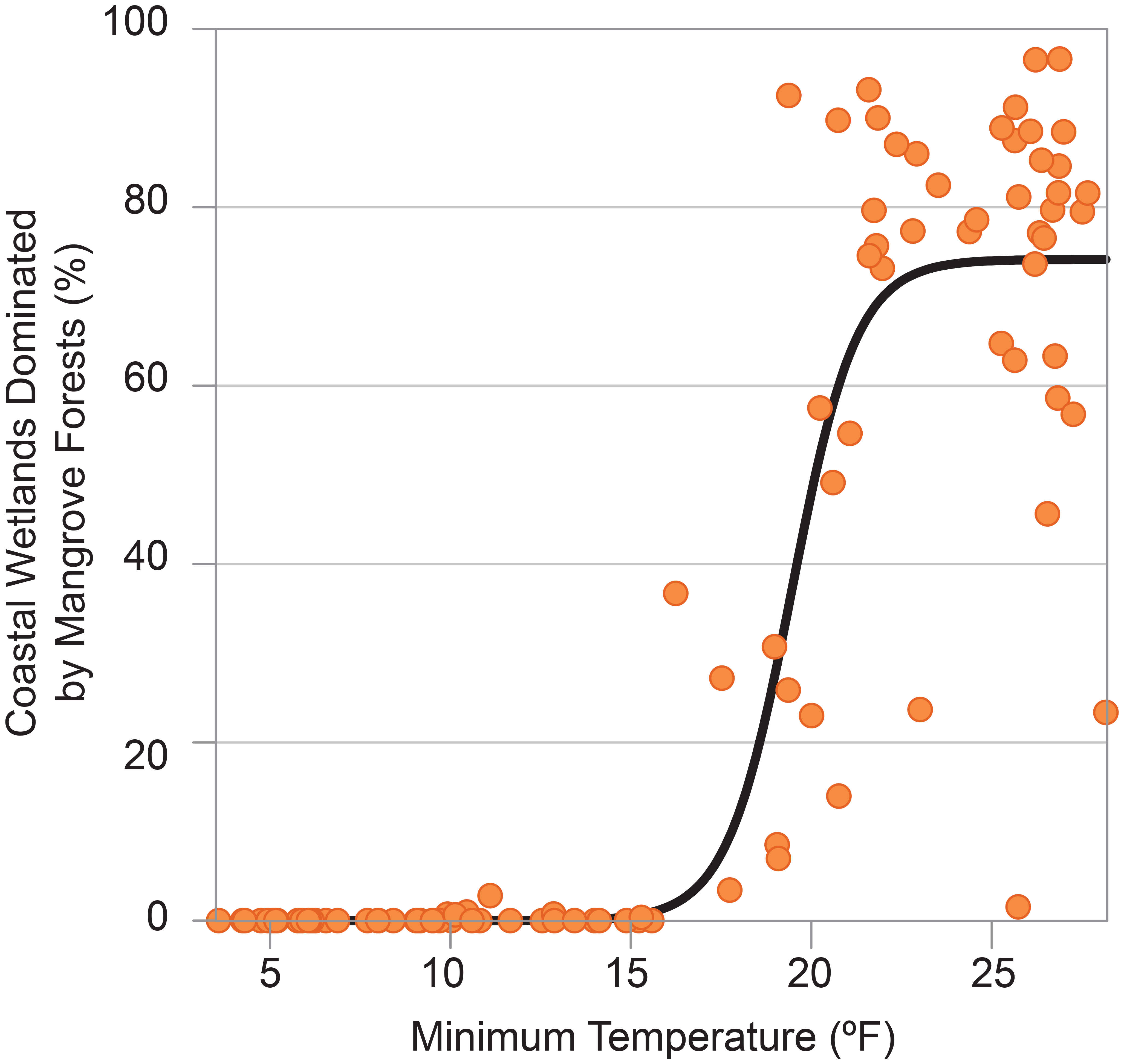
Winter air temperature extremes (for example, freezing and chilling events) constrain the northern limit of many tropical and subtropical species.30,48,127,132,135,138,139,140,141,142,143,144,145,148,149,150,152,166,167,168,169,170,172,173,174,175,176,177,178 In the future, warmer winter temperatures are expected to facilitate the northward movement of cold-sensitive species, often at the expense of cold-tolerant species.132,135,142,145,149,150,152,166,169,173,179 Certain ecosystems are located near thresholds where small changes in winter air temperature regimes can trigger comparatively large and abrupt landscape-scale ecological changes (i.e., ecological regime shifts).135,145,152
Changing fire regimes are expected to have a large impact on natural systems. Fire has historically played an important role in the region, and ecological diversity in many southeastern natural systems is dependent upon fire.115,116,134,189 In the future, rising temperatures and increases in the duration and intensity of drought are expected to increase wildfire occurrence and also reduce the effectiveness of prescribed fire.3,4,5,6
Hurricanes and rising sea levels are aspects of climate change that will have a tremendous effect on coastal ecosystems in the Southeast. Historically, coastal ecosystems in the region have adjusted to sea level rise via vertical and/or horizontal movement across the landscape.125,129,200,201 As sea levels rise in the future, some coastal ecosystems will be submerged and converted to open water, and some coastal ecosystems will move inland at the expense of upslope and upriver ecosystems.203,204 Since coastal terrestrial and freshwater ecosystems are highly sensitive to increases in inundation and/or salinity, sea level rise will result in the comparatively rapid conversion of these systems to tidal saline habitats. In addition to sea level rise, climate change is expected to increase the impacts of hurricanes; the high winds, storm surges, inundation, and salts that accompany hurricanes will have large ecological impacts to terrestrial and freshwater ecosystems.209,210
Climate change is expected to intensify the hydrologic cycle and increase the frequency and severity of extreme events. Extreme drought events are expected to become more frequent and severe. Drought and extreme heat can result in tree mortality and transform southeastern forested ecosystems.217,218,219,220,221,222,223 Drought can also affect aquatic and wetland ecosystems.224,225,226,227,228,229,232 Extreme rainfall events are also expected to become more frequent and severe in the future. The prolonged inundation and lack of oxygen that result from extreme rainfall events can also result in mortality and large impacts to natural systems.233 In combination, future increases in both extreme drought and extreme rainfall are expected to transform many southeastern ecosystems.
Warming ocean temperatures due to climate change are expected to have a large effect on marine and coastal ecosystems.234,235,236 Many species are sensitive to small changes in ocean temperature; hence, the distribution and abundance of marine organisms are expected to be greatly altered by increasing ocean temperatures. For example, the distribution of tropical herbivorous fish has been expanding in response to warmer waters, which has resulted in the tropicalization of some temperate marine ecosystems and decreases in the cover of valuable macroalgal plant communities.179 A decrease in the growth of sea turtles in the West Atlantic has been linked to higher ocean temperatures.237 The impacts to coral reef ecosystems have been and are expected to be particularly dire. Coral reef mortality in the Florida Keys and across the globe has been very high in recent decades, due in part to warming ocean temperatures, nutrient enrichment, overfishing, and coastal development.240,241,242,243,244 Coral elevation and volume in the Florida Keys have been declining in recent decades,245 and present-day temperatures in the region are already close to bleaching thresholds; hence, it is likely that many of the remaining coral reefs in the Southeast will be lost in the coming decades.246,247 In addition to warming temperatures, accelerated ocean acidification is also expected to contribute to coral reef mortality and decline.248,249
Major uncertainties
In the Southeast, winter temperature extremes, fire regimes, sea level fluctuations, hurricanes, extreme rainfall, and extreme drought all play critical roles and greatly influence the distribution, structure, and function of species and ecosystems. Changing climatic conditions (particularly, changes in the frequency and severity of climate extremes) are, however, difficult to replicate via experimental manipulations; hence, ecological responses to future climate regimes have not been fully quantified for all species and ecosystems. Natural ecosystems are complex and governed by many interacting biotic and abiotic processes. Although it is possible to make general predictions of climate change effects, specific future ecological transformations can be difficult to predict, especially given the number of interacting and changing biotic and abiotic factors in any specific location. Uncertainties in the range of potential future changes in multiple and concurrent facets of climate and land-use change also affect our ability to predict changes to natural systems.
Description of confidence and likelihood
There is high confidence that climate change (e.g., changing winter temperatures extremes, changing fire regimes, rising sea levels and hurricanes, warming ocean temperatures, and more extreme rainfall and drought) will very likely affect natural systems in the Southeast region. These climatic drivers play critical roles and greatly influence the distribution, structure, and functioning of ecosystems; hence, changes in these climatic drivers will transform ecosystems in the region and greatly alter the distribution and abundance of species.
Key Message 4: Economic and Health Risks for Rural Communities
Rural communities are integral to the Southeast’s cultural heritage and to the strong agricultural and forest products industries across the region. More frequent extreme heat episodes and changing seasonal climates are projected to increase exposure-linked health impacts and economic vulnerabilities in the agricultural, timber, and manufacturing sectors (very likely, high confidence). By the end of the century, over one-half billion labor hours could be lost from extreme heat-related impacts (likely, medium confidence). Such changes would negatively impact the region’s labor-intensive agricultural industry and compound existing social stresses in rural areas related to limited local community capabilities and associated with rural demography, occupations, earnings, literacy, and poverty incidence (very likely, high confidence). Reduction of existing stresses can increase resilience (very likely, high confidence).
Description of evidence base
Analysis of the sensitivity of some manufacturing sectors to climate changes anticipates secondary risks associated with crop and livestock productivity.64,255
Multiple analyses anticipate that energy- or water-intensive industries could face water stress and increased energy costs.8,64,255,256
A large body of evidence addresses the sensitivity of many crops grown in the Southeast to changing climate conditions including increased temperatures, decreased summer rainfall, drought, and change in the timing and duration of chill periods.7,35 Extensive research documents livestock sensitivity to heat stress.7
Multiple lines of evidence indicate that forests are likely to be impacted by changing climate, particularly moisture regimes and potential changes in wildfire activity.191,195,272,274 There is extensive research on heat-related illness and mortality among those living and working in the Southeast. While there is more evidence focused on urban areas, limited research has identified higher levels of heat-related illness in rural areas.280,281 Research on occupational heat-related mortality identifies some of the Nation’s highest levels in southeastern states.282 Computer model simulations of heat-related reductions in labor productivity anticipate the greatest losses will occur in the Southeast. However, these models do not account for adaptations that may reduce estimated losses.35,64 By the end of the century, mean annual electricity costs are estimated at $3.3 billion each year under RCP8.5 (model range: $2.4 to $4.2 billion; in 2015 dollars, undiscounted) and mean $1.2 billion each year under RCP4.5 (model range $0.9 to $1.9 billion; in 2015 dollars, undiscounted).35
Rural communities tend to be vulnerable due to factors such as demography, occupations, earnings, literacy, and poverty incidence.8,9,10,250,283,284,305 Reducing the stress created by such factors can improve resilience.9,284 The availability and accessibility of planning and health services to support coping with climate-related stresses are limited in the rural Southeast.288,289
Major uncertainties
There are limited studies documenting direct connections between climate changes and economic impacts. Models are limited in their ability to incorporate adaptation that may reduce losses. These factors restrict the potential to strongly associate declines in agricultural and forest productivity with the level of potential economic impact.
Projections of potential change in the frequency and extent of wildfires depend in part on models of future population growth and human behavior, which are limited, adding to the uncertainty associated with climate and forest modeling.
Many indicators of vulnerability are dynamic, so that adaptation and other changes can affect the patterns of vulnerability to heat and other climate stressors over time. Limited studies indicate concerns over the planning and preparedness of capacity at local levels; however, information is limited.
Projected labor hours lost vary by global climate model, time frame, and scenario, with a mean of 0.57 and a model range of 0.34–0.82 billion labor hours lost each year for RCP8.5 by 2090. The annual mean projected losses are roughly halved (0.28 billion labor hours) and with a model range from 0.19 to 0.43 billion labor hours lost under RCP4.5 by 2090.35
Description of confidence and likelihood
There is high confidence that climate change (e.g., rising temperatures, changing fire regimes, rising sea levels, and more extreme rainfall and drought) will very likely affect agricultural and forest products industries, potentially resulting in economic impacts. There is high confidence that increases in temperature are very likely to increase heat-related illness, deaths, and loss of labor productivity without greater adaptation efforts.